
VLOOKUP Formula in Excel: A Step-by-Step Guide with Examples
Introduction to VLOOKUP
VLOOKUP Formula in Excel is one of Excel’s most powerful and widely used functions. The full form of VLOOKUP is Vertical Lookup. It is used to search for a value in the first column of a table and return a corresponding value from another column in the same row.
Syntax of VLOOKUP
=VLOOKUP(lookup_value, table_array, col_index_num, [range_lookup])
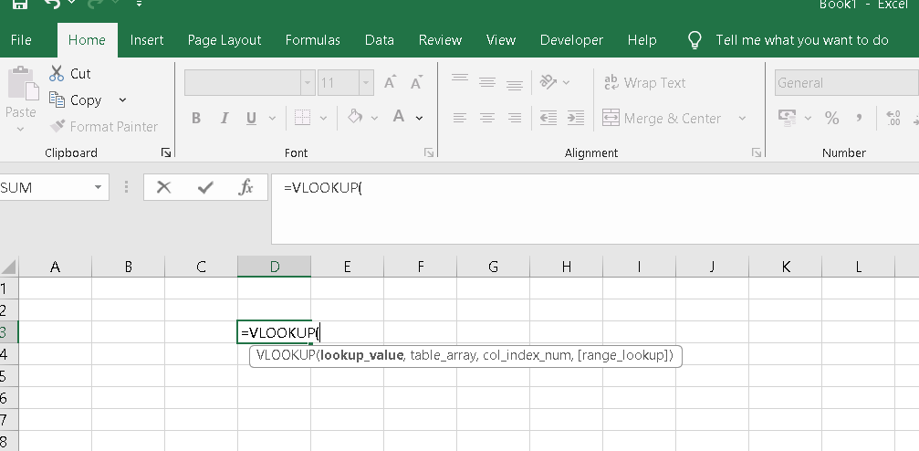
Explanation of Arguments:
- Lookup_value – The value you want to search for in the first column of your dataset.
- Table_array – The range of cells containing the data, including both the column you search in and the column you want to retrieve data from.
- Col_index_num – The column number in the table from which to return a value.the first column of values in the table is column 1.
- Range_lookup – TRUE (Approximate Match) or FALSE (Exact Match). In most cases, FALSE is used to find an exact match. You Can also use 0 for Exact Match and 1 for Approximate Match.
How to use VLOOKUP: Step-by-Step Guide
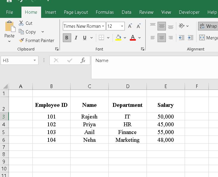
Step 1: Prepare Your Data
Before applying the VLOOKUP formula, ensure your data is organized properly. The column you are searching in (the first column of the table) must contain unique values.
Example Dataset
Step 2: Apply the VLOOKUP Formula
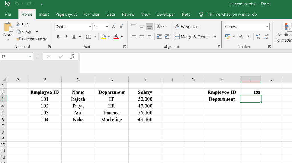
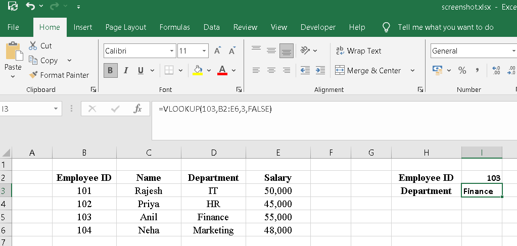
Now, let’s say you want to find the department of employee ID 103.
Enter the formula: Now, let’s say you want to find the department of employee ID 103.
- Click on the cell where you want the result to appear (e.g., I3).
- Enter the formula:
- =VLOOKUP(103, B2:E6, 3, FALSE)
- Press Enter
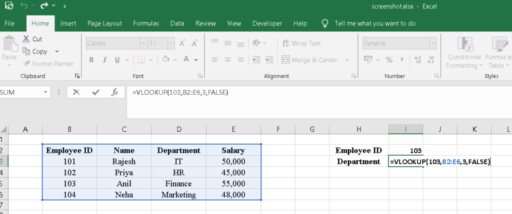
Explanation of the Formula:
- 103 → The lookup value (Employee ID).
- B2:E6 → The data range must include both the Employee ID and Department columns.
- 3 → The 3rd column in the range (Department).
- FALSE → An exact match is required.
Step 3: Check the Result
The result in I3 will be Finance (as Employee ID 103 belongs to Finance
VLOOKUP with a Dynamic Lookup Value
Instead of entering the lookup value manually, you can reference another cell.
Type 103 in cell I2.
In I3, use the formula:
=VLOOKUP(I2,B2:E6,3,FALSE)
Now, whenever you change the value in I2, the result in I3 will automatically update.
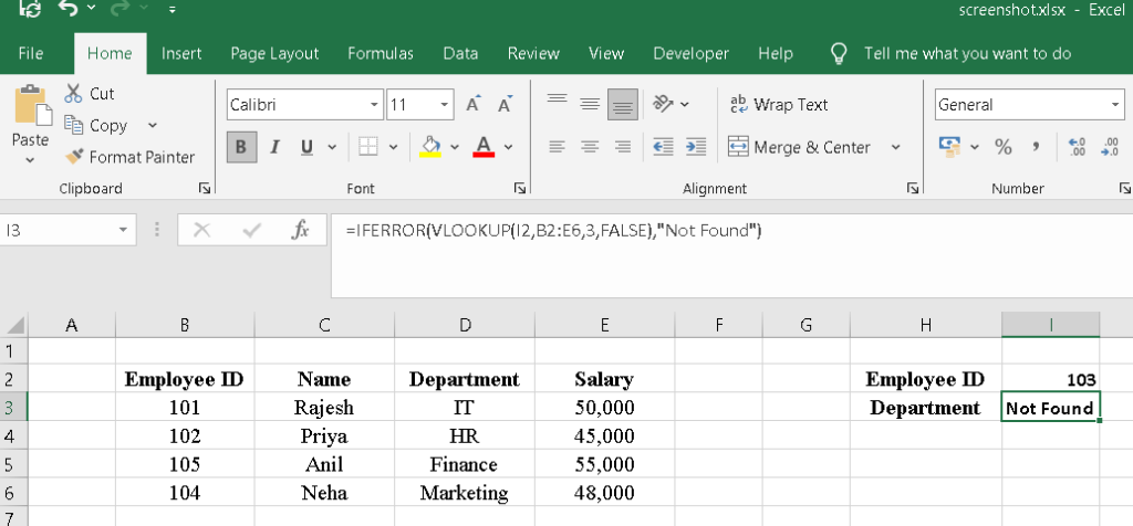
Handling Errors
If a value is not found, VLOOKUP returns a #N/A error. To avoid this, use IFERROR:
=IFERROR(VLOOKUP(I2,B2:E6,3,FALSE), “Not Found”)
This will return “Not Found” instead of an error.
VLOOKUP with Approximate Match
If you are looking for a range-based value, use TRUE as the last argument.
Example: You have a grading system:
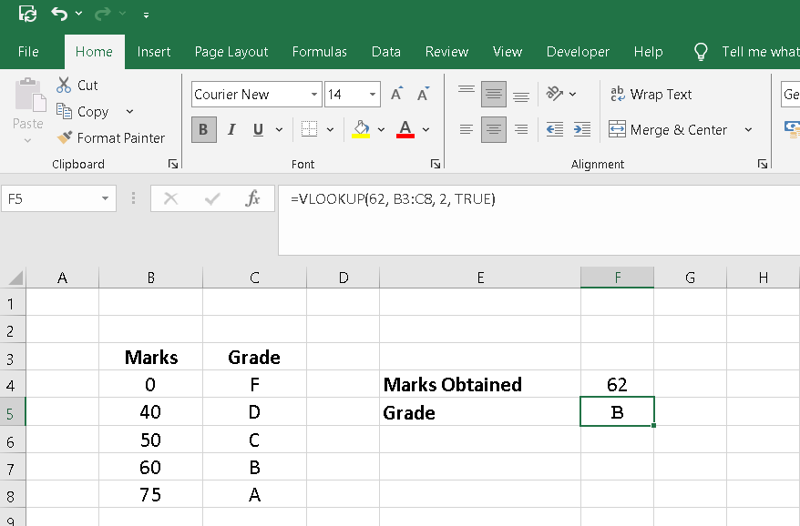
To find the grade for a student who scored 62, use:
=VLOOKUP(62, B3:C8, 2, TRUE)
VLOOKUP finds the largest value that is less than or equal to 62, which is 60, and returns B.
Common Issues and Fixes
| Issue | Solution |
| #N/A Error | Check if the lookup value exists in the first column. |
| Incorrect Result | Ensure the column index number is correct. |
| #REF! Error | Ensure the column index number does not exceed the number of columns in the range. |
| #VALUE! Error | Check if the formula arguments are correctly entered. |
Tips for Using VLOOKUP Effectively
-
Use Absolute References (
$B$2:$E$6) to keep the table range fixed. Using absolute references, Vlookup will search the entire range for the look up value. -
Sort Data in Ascending Order for an approximate match.
-
Use INDEX & MATCH as an alternative for more flexibility.INDEX & MATCH formula in Excel is much flexible.
Conclusion
VLOOKUP is a powerful function that helps in data retrieval in Excel. By following this step-by-step guide, you can efficiently use this formula for various data lookups. However, if you find any issue related to the VLOOKUP Function, you can ask by commenting on this post. We will try our best to resolve your issue as soon as possible.
Thanks